Abstract

This paper provides a broad overview of the issue of rising inequality, and it builds an international and multidimensional taxonomy of economic inequality. We use a hierarchical cluster analysis, which enables us to identify five groups of countries with distinctive economic inequality features, which show that, despite national and regional specificities, both developed and developing countries face important hurdles in reducing social and economic disparities. The resulting classification may be useful to map out the various national realities of economic inequality across countries. The results suggest that a one-size-fits-all international strategy should be avoided in order to address the different patterns of inequality that we have identified around the world. Still, it is crucial to acknowledge the importance of the particularities of each cluster and each geographic region regarding a complex and multidimensional phenomenon, which has become a global challenge for the 21st century.

Keywords: Cluster Analysis; Country Classification; Economic Inequality; Polarization, and Sustainable Development

Resumen

Este artículo ofrece una revisión del creciente problema de la desigualdad y construye una taxonomía internacional y multidimensional de la desigualdad económica. Se utiliza un análisis jerárquico de conglomerados que nos permite identificar cinco grupos de países con características distintivas de desigualdad económica, que muestran que, a pesar de las especificidades nacionales y regionales, tanto los países desarrollados como los países en desarrollo se enfrentan a importantes dificultades para reducir las disparidades sociales y económicas. La clasificación resultante puede ser útil para trazar un mapa de las distintas realidades nacionales de la desigualdad económica entre países. Los resultados sugieren que debería evitarse una estrategia internacional de “talla única” para abordar los diferentes patrones de desigualdad que hemos identificado en todo el mundo. Aun así, es crucial reconocer la importancia de las particularidades de cada conglomerado y de cada región geográfica en relación con un fenómeno complejo y multidimensional que se ha convertido en un reto global para el siglo XXI.

Palabras clave: Análisis de conglomerados, Clasificación de países, Desigualdad económica, Polarización, y Desarrollo sostenible.

1. Introduction

Inequality is a multidimensional and complex phenomenon: a prism through which multiple development problems emerge, being a complex issue that requires global solutions. In accordance with the United Nations’ (UN) 2030 Agenda for Sustainable Development, and the unprecedent challenge of Covid-19 pandemic for global development, “the achievement of inclusive and sustainable economic growth [...] will only be possible if wealth is shared and income inequality is addressed” (UN, 2015, p. 8).

Accordingly, the Sustainable Development Goals (SDG) try to respond to the concerns regarding equality not only with a standalone objective in mind (the SDG 10 “reduce inequality within and among countries”), but also as a way to address cross-cutting issues. In this regard, reducing inequalities implies interaction with other development concerns related to poverty, conflict, gender, health, nutrition, education, and environmental sustainability, among others (Gaventa, 2016).

While this paper acknowledges the existence of different dimensions that are connected to inequality, it focuses on global “economic inequalities” through the prism of their different features that point out a key current concern: the growing divide between the rich and the poor.

We propose a complementary approach to assessing the SDG 10 by means of a hierarchical cluster analysis. The aim of this article is build an international and multidimensional taxonomy of economic inequalities that considers five main dimensions of income and wealth (household income, wealth growth of the rich, income growth of the poor, income concentration, and State’s capacity to tackle inequalities) in order to identify groups of countries with distinctive inequality characteristics. We focus on the mid-2010s, which includes the immediate aftermath of the last Great Recession and the beginning of a period of recovery.

In order to build a realistic taxonomy, we deal with a key concern: the search of the “true” value of global economic inequality and its distribution among countries over time (Milanovic, 2012 and 2016; Lakner and Milanovic, 2016). We assume that economic inequality is intrinsically a multifaceted concept that includes two major components: the distribution of income and financial wealth among individuals, and the capacity of the State to alleviate social disparities. Therefore, the analysis of inequality should not be focused on a single yardstick because this may lead to confusion and misinterpretation. Consequently, we build an international taxonomy that takes into consideration key estimates of inequality and poverty. Our aim is to comprehensively address the intricacies of income (and wealth) disparities across countries. The main results allow us to identify five groups of countries, each exhibiting unique characteristics of economic inequality. This demonstrates that, irrespective of national and regional specificities, both developed and developing countries face significant challenges in reducing social and economic disparities.

The paper is structured as follow: After this introduction, section two briefly reviews the literature on the macroeconomics of income inequality, the recent approaches in measuring inequality, and the importance of bridging the dots between national and household income. Section three explains the methodology we employ to construct a multidimensional taxonomy of international economic inequalities. This includes a discussion of the dimensions and variables used in the analysis, as well as the statistical procedure of cluster analysis. Section four presents the main empirical results of our piece of research. Finally, section five addresses conclusions.

2. State of the art

2.1. Macroeconomics of income inequality

Inequalities have been part of a long-standing preoccupation for social scientists (Rawls, 1971; Roemer & Trannoy, 2015). There seems to be a shared understanding about the diagnosis that exceeding certain limits of inequality may foster “social disintegration, unrest and violence” (Fleurbaey & Klasen, 2016, p. 175). Long-term trends suggest that high peaks of inequality have been curbed by warfare, revolution, State collapse, and plagues (Scheidel, 2016). For instance, before World War, II John Maynard Keynes warned that inequalities reached unprecedented high levels —although he did not deny certain room for inequality. In his words:

I believe that there is social and psychological justification for significant inequalities of incomes and wealth, but not for such a large disparity as exists today (Keynes 1936, p. 374).

Interestingly, while war aversion has risen since the World War II, there is evidence of growing inequalities around the word over the last decades, hand in hand with the expansion of financial globalization (Mueller, 2009). At the same time, there is a growing mistrust on the expansion of capital markets and their effects on macro instability and the deterioration of productive capacities (Mundell, 1963). These mistrusts have gained momentum throughout the extensive use of market-based financing as a substitute for bank financing (Brei et al., 2018). Yet, inequalities continue to widen, particularly in those countries with weak institutional capacities, leading into an emerging pattern where inequality is strongly linked with less sustained growth (Ostry, Loungani & Berg, 2019). The explanation of inequality, therefore, involves a complex set of interactions that emphasizes, among others, the role of global interdependencies and the contradictions of the dominant economic and cooperation systems, as suggested by critical approaches, such as the dependency theory and the world-system theory (dos Santos, 2011; Wallerstein, 2004; Arrighi, 2007; Domínguez, 2014).

Furthermore, on the empirical perspective, there are two major story lines of global inequality –broadly disseminated and discussed in a different policy fora over the last 10 years– which are closely interrelated. On the one hand, it is argued that inequality is steadily on the rise under capitalism due to the evolution of the capital-income ratio and technological progress. The assumption behind this approach is that the average annual rate of return of capital –ceteris paribus– is greater than the Gross Domestic Product (GDP)’s rate of growth (Piketty, 2014). According to this view, inequality is very likely to occur through the unequal distribution of income going to capital, measured as a percentage of national income. While this might allow an increase of the labor-income ratio, inequality rises to a greater extent because of the growing share of capital in GDP. Furthermore, this involves a reduction of capital productivity and the decline in the labor income share, as it has been verified in a cross-country analysis over recent decades (Ibarra and Ros, 2019). Therefore, if this trend continues, the shift of income to owners of capital –and thus, the increase of inequality– is expected to continue.

On the other hand, the second story line suggests that inequality moves in waves or cycles influenced by “benign forces” (e.g., redistribution, labor unions, and widespread education, among others) and “malignant forces” (wars, epidemics, hyperinflation, etc.) (Milanovic, 2016 & 2019). This approach relies on Kuznets’ interpretation upon the study of long-term changes in income distribution. Based on this, Milanovic (2016) identifies three phases of inequality from the pre-Industrial Revolution period onwards. In the first phase, prior to 1760, inequality moved ‘around a basically fixed average income level’ (Milanovic, 2016, p. 50). In the second phase, from the Industrial Revolution to the Reagan-Thatcher Revolution, there was a long wave of inequality, which included both a sharp increase of inequality after the Industrial Revolution period with a peak at the turn of the 20th century, and a downward trend after the World War I. In the last phase, from the end of the 1980s onwards, inequality mainly increased due to the emergence of a ‘new (second) technological revolution,’ in the context of the rapid spread of economic and financial globalization.

Both story lines on inequality share similar features, such as the interest in the role of technological progress and capital concentration. Nonetheless, they offer different normative conclusions: the first approach considers that the best –“fairest and potent”– way to redistribute income is through progressive income taxation, while the second approach believes that a more realistic manner –in political terms– would be through equalizing endowments and deconcentrating capital ownership. These include, inter alia, progressive taxation, and inheritance taxation, among others.

Yet, at the heart of the discussion a crucial question remains: what is the ‘true’ level of economic inequality within and across countries?

2.2 Measurement of inequality: recent approaches

Knowledge about the evolution of inequality over time has improved thanks to the development of several databases, which have enhanced the availability, quality, and comparability of international data. These efforts include a variety of specialized agencies, organizations, and individual scholars. However, there remains an outstanding issue in terms of data consistency, leading to discrepancies in the ‘levels and trends of inequality obtained from each database’ (UNDESA 2018, p. 1). Examples of different sources of information are the UNU-WIDER’s World Income Inequality Database (WIID), the OECD’s Income Distribution Database (IDD), the Poverty and Equity Database provided by the World Bank, the Global Consumption and Income Project (GCIP), the Luxembourg Income Study and Wealth Study Databases (LIS and LWS), and the collection of global wealth reports published by the Credit Suisse Research Institute.

More specifically, the specialised literature on income inequality is trying to connect “the dots between macroeconomics and the distribution of income” (Atkinson, 2015, p. 100). This refers to the information gap created by the constraints and omissions that household surveys impose upon the understanding of income inequality and poverty. As a direct consequence, there is a growing body of literature particularly interested in analyzing developed countries with a long-term perspective (Atkinson, 2007; Atkinson, Piketty & Saez, 2011; Piketty, 2014; Atkinson & Bourguignon, 2015).

The contemporary interest in inequality mainly focuses on the study of distribution of income and wealth among individuals (Stiglitz, 1969). Nonetheless, these studies have used income tax data, which is an extremely sensitive source of information for a wide range of developing countries, both politically and institutionally (Kaldor, 1980). This constraint does not allow scholars and practitioners to access comparable cross-country tax data, which is essential for understanding the structure and complexity of global income disparities. These data might provide key insights on how high incomes –especially the share of wealth owned by the top 0.1%– influence the distribution of income over time. This is of concern particularly in a context where the upper tail of the distribution seems somewhat underestimated over the recent years. In fact, there is a virtual unanimity regarding the existence of a highly skewed income distribution (Alvaredo et al., 2018; UNDP, 2019).

In this regard, the method described by Lakner and Milanovic (2016), following Atkinson (2007), addresses the tendency to underreporting top incomes in household surveys and their discrepancy with national accounts. This involves spreading:

[…] the discrepancy between national accounts and household surveys evenly across the distribution, but for the very top through the elongation of the distribution, by using a Pareto interpolation, the so-called “proportional adjustment with Pareto tail” (Lakner and Milanovic 2016, p. 21).

By allocating the excess of income recorded in national accounts over the upper part of the income distribution in household surveys, it is possible to obtain a more realistic picture of the phenomenon of inequality and poverty.

Atkinson (2015) provides a useful guide to explain how to connect the dots between national income and household income. Figure 1 gives an overview of the complexity of this adjustment, establishing some of the links between the estimates offered by each source of income data. The figure reflects the idea that the categories under analysis are not necessarily equivalent, and it identifies structures and agents that influence the main determinants of household income. Likewise, it makes emphasis on the importance of having a broad approach when dealing with income inequality from a global perspective. One important message in this framework is that the connections between income components and outcomes are not straightforward or even easy to estimate. At best, the estimates of income that arise from the household sector are an imperfect matching of a complex interaction of influencing formal, and informal factors.

Figure 1. From national income to household income in a global and interdependent world

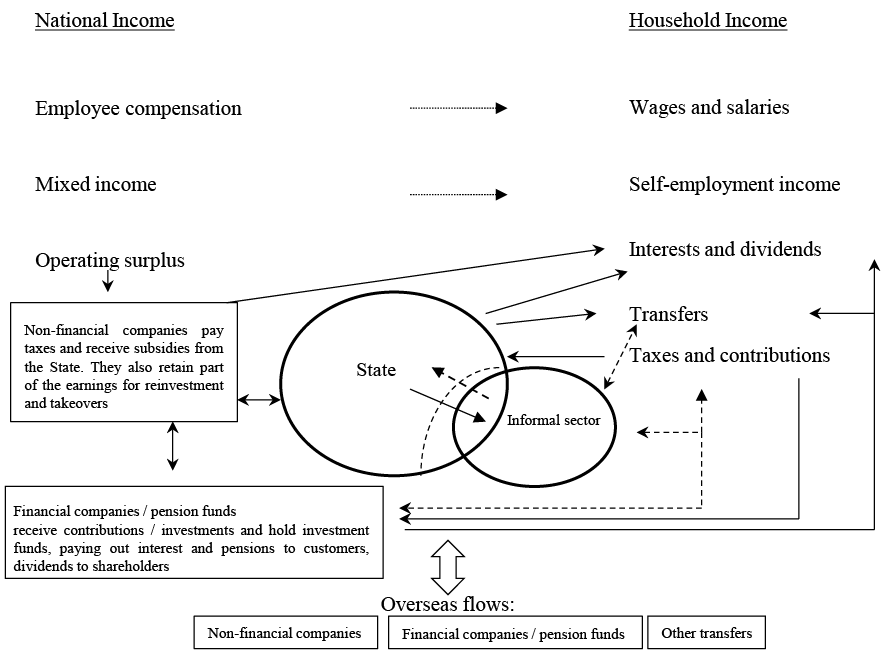
Source: Based on Atkinson (2015)

Moreover, Atkinson (2015) identifies recognizable features between national and household incomes. For instance, the possible connections between employee compensations, wages, and salaries (Figure 1). Similarly, his framework of analysis introduces key institutional elements, such as the State and financial and nonfinancial companies. The former is perceived as the main agent of change that serves as a filter through which households receive transfers and pay taxes. In this process, the State can provide access to fundamental rights (infrastructure, education, and health, among others). Inevitably, this involves the creation of assets that are determinant factors in obtaining a more sustainable development process. Obviously, the counterweight to this are domestic and foreign debts that constrain the room for maneuver and the potential to expand people’s choices over time. The former is the consequence of broader strategic issues in which the connection and inter-dependence with financial and nonfinancial services in an open economy stimulate a set of income supplements (i.e. corporate earnings, financial dividends, investments, pensions, etc.).

Furthermore, the importance of the State’s capability to reduce income inequalities should not be underestimated. It is here where the greatest differences emerge between developed and developing countries. In the first case, the expansion of income is the result of a process in which the State has been a fundamental stakeholder, by providing institutional structures for high-quality development at both domestic and international levels (Chang, 2011). In this process, developed countries have created more equitable and efficient tax systems, which go hand in hand with mutually reinforcing interactions between employment and social protection policies. In contrast, in developing countries, the informal sector performs some of the State’s tasks, in particular those related to income redistribution. In part, this reflects the structural institutional failure that prevents these economies from taking a qualitative leap towards greater socio-economic development. The duality between the State and the informal sector is a distinctive feature of developing countries.

Figure 1 also shows the complex connections between the different categories that affect national and household income. This may be seen as flows of transactions –shown by solid and dashed lines–, by going both ways: through the State or the informal sector, depending on whether households are fully integrated into the formal economy. These two main sectors (formal and informal) receive and pay transfers and contributions. Over time, this duality has become more complex and multidimensional. Not only the informal sector does take a prominent position in developing countries (i.e. through informal employment or illicit activities), but also there is also evidence of closer integration of informal and formal sectors within an international context which faces difficulties in creating and securing permanent jobs through economic growth (La Porta & Shleifer, 2014). Moreover, while in developing countries the informal sector serves as a basic social protection system in periods of crisis, people in developed countries depend on social protection policies, —such as unemployment insurance benefits. Both types of schemes have advantages and disadvantages for people’s choices. In developing countries, the informal sector provides employment in the short-term –low-productivity jobs combined with low salaries–, and the consequent access to basic services. Certainly, this scheme offers poor coverage in terms of job security and good working conditions, and it has a negative impact on the creation of fair and efficient tax systems, which favors the fragmentation of the internal market and the lack of social and institutional cohesion. In developed countries, the potential gains and opportunities of social protection programs may be affected by the lack of secure jobs in the short-and-medium terms. To a large extent, this depends on the capacity of these countries of fostering more productive development policies. In both cases, there is a consistent social coverage policy through traditional family and community support structures.

Formal and informal sectors also have a connection with financial and nonfinancial services. Wherever possible, financial and nonfinancial institutions provide mechanisms through which to energize the circular flow of income in an open economy. These mechanisms include not only unilateral transfers of income from abroad, —such as remittances, —but also the management of a growing pool of retirement savings, or even, the transfer of illicit financial flows (OECD, 2014).

All in all, Figure 1 simplifies the complex set of aspects that affect household income. As stated by Atkinson (2015, p. 102), ‘total household income is considerably less than total national income.’ This includes the issue of concentration of income at the very top, the widening gap between the rich and the poor in a dynamic and competitive global setting, and the role of the State in tackling inequality. All of them are essential aspects for measuring inequality trends, as we will see below.

3. Methodology for building a multidimensional taxonomy of international economic inequalities

3.1 Dimensions, variables, and period of analysis

Since we are interested in building a multidimensional taxonomy of economic inequalities across countries, we identify five dimensions that are relevant for reproducing these inequalities. Thus, we try to overcome a single measurement of economic inequality, which inevitable reflects a normative preference, as suggested by Atkinson (1970) and Ravallion (2018). However, we also add the main narratives surrounding the problem of inequality. We acknowledge that global economic inequality is a multidimensional issue transcending income and wealth, and thus, our analysis is a limited attempt to provide a classification of countries. However, we provide a multifaceted picture of economic inequalities with mutually reinforcing and complementing components of this growing concern. Thus, we go beyond single yardsticks.

In order to build our international taxonomy, we place special emphasis on five dimensions: i) adjusted household income, ii) wealth growth of the rich, iii) income concentration, iv) income growth of the poor, and v) State’s capacity to tackle inequalities. As argued, these dimensions account for the dominant explanations of economic inequality. On the one hand, we consider the role of income disparities between the extremes of the income distribution. On the other hand, we also consider income concentration, which primarily reflects changes in inequality within the middle portion of the income distribution. Similarly, our approach includes the growth of the lowest income deciles, by explaining the progress of countries towards lower inequality. Additionally, the component of financial wealth, which is typically omitted in cross-country inequality comparisons, is included here, by providing a comprehensive view of this issue. Lastly, the State’s capacity to increase public revenues is essential for implementing policies in order to reduce inequality.

Regarding the period of analysis, the proxies are computed for 2015, which includes the immediate aftermath of the last Great Recession and the beginning of a period of recovery. In doing so, it is also very important to say that these proxies offer the best information available to create a global database of economic inequality through different lenses. Certainly, there are other proxies for each dimension that have been used in different studies. Nonetheless, they provide a certain bias towards advanced and Western economies. Therefore, there is an urgent need to provide analysis of this problem from a comprehensive perspective with the inclusion of countries of the Global South. In this sense, this is an approach that considers relevant dimensions related to the problem of economic inequalities, in line with the previous literature. Moreover, the article has sought to offer a global perspective based on a broad sample of countries, by encompassing both developed and developing nations. Nonetheless, it is unavoidable to omit some countries due to the absence of data.

Table 1 shows the dimensions, variables, periods, and sources used for the 101 countries, which are included in our empirical estimation.

Table 1. Dimensions and variables of analysis

SDG	Dimensions	Proxies	Sources	Period
Reduce inequality within and among countries (SDG 10)	Adjusted household income	Household income (means level of income, 2011 PPP) per capita adjusted by surveys and national accounts (Income_pc_adj)	World Bank (2020) and Global Consumption and Income Project (GCIP) (Lahoti et al. 2016)	2015
	Wealth growth of the rich	Change in the proportion of adults with more than 100,000 USD wealth (percentage points) (Growth_rich)	Credit Suisse Research Institute (2012 and 2015)	2012-2015
	Income growth of the poor	Growth rates of household expenditure or income per capita among the bottom 40 per cent of the population (%) (Growth40)	World Bank (2020)	Last available estimate for the period 2013-2017
	Income concentration	Palma ratio adjusted by surveys and national accounts (Palma)	World Bank (2020) and Global Consumption Income Project (GCIP) (Lahoti et al. 2016)	2015
	State’s capacity to tackle inequalities	Tax revenue as share of GDP (Tax_revenue)	ICTD / UNU-WIDER Government Revenue Dataset (2018)	2015

Source: Authors.

i) Household income

One important point regarding this dimension has to do with the idea of providing plausible estimates of income inequality across countries, by involving the correction of household survey data, based on the scale invariance axiom –which assumes that incomes are equally distributed within country deciles over time. We try to partially correct this bias, by using standardized levels of income based on surveys and national accounts estimates (Niño-Zarazúa et al., 2017). The inclusion of the size of the income distribution is relevant to capture the contribution of each country on a global scale.

In particular, we use the Global Income Dataset (GID) provided by the Global Consumption and Income Project (GCIP) due to its capacity to create an ̒ecumenical approach’ that integrates different sources, such as the EU-SILC database, the LIS, the SEDLAC database, the UNU-WIDER World Income Inequality Database, the World Bank’s Povcalnet database, and Branko Milanovic’s WYD database (Lahoti, et al, 2016: 6). In contrast to other global income datasets (for example, Lakner and Milanovic, 2016), GID employs a ‘standardized income concept’ which facilitates cross-country comparisons over time and provides estimates of monthly real income in almost all countries for the period 1960-2015.

We use data in mean levels of income by country in terms of the 2011 purchasing power parity (PPP) dollars. We argued that income levels provide the basis for cross-country comparison of economic inequality for their capacity to reveal the scale of income across countries over time.

According to the GID, as Figure 2 shows, the Lorenz curves for the global income distribution between 1990 and 2015 indicate that there has been a decrease in global inequality (between nations), mainly through the economic performance of China and India, as suggested by Kanbur (2019).

Figure 2. Global income distribution: Lorenz curve 1990–2015

Source: Authors, based on data from the World Bank (2020) and the Global Consumption Income Project (GCIP) (2016).

ii) Wealth growth of the rich

The concentration of wealth in the hands of the rich is a controversial issue worldwide because of its implications on global inequality, in particular in terms of the growing gap between the rich and the poor within and between countries. This debate has been propelled by the reports annually published by Oxfam International since 2010 (which are based on the statistics provided by the Forbes billionaires’ lists and the Credit Suisse Global Wealth Reports and Databooks), as well as the World Inequality Database elaborated by the Paris School of Economics (which has some constraints in terms of geographical coverage across countries).

Despite the economic differences between wealth (which is a stock variable) and income (which is a flow variable), they are key complementary features of economic inequality (Keeley, 2015). Wealth is particularly relevant for understanding the huge asymmetries between the World’s billionaires and the ultra-poor.

We proxy this dimension by means of the variation (in percentage points), between 2012 and 2015, of the proportion of adults with more than 100,000 USD wealth.

iii) Income concentration

The Gini coefficient is one of the most common measures of inequality, which —along with other measures, such as the Theil index— are “Lorenz consistent” (Fields, 2002). However, Gini coefficient tends to overlook the tails of the distribution and is insensitive to high levels of inequality (Josa & Aguado, 2020). According to Palma (2014), there has been an obsession regarding the analysis of the changes occurring in the middle 50% of the distribution, which are shown to be relatively stable across and within countries over time. All this adds up to a certain reluctance to shift the focus to the bottom 40% and the top 10%, where inequality seems to be more relevant. Accordingly, the Palma ratio is an alternative measure to the Gini index, despite the fact that some critics suggest that changes in the extremes of the income distribution can only be part of “an empirical regularity that may not hold in the future” (Cobham, Schlögl & Sumner, 2016: 28). Given the evolution and the features of rising inequality at global scale, the Palma ratio seems to be the most appropriate proxy for our analysis.

iv) Income growth of the poor

Fostering the income growth of the poorest people across countries is necessary in order to both eradicate extreme poverty (as stated by the first SDG) and to reduce income inequalities (SDG 10).1 The literature suggests that improvements in shared prosperity, particularly for the poorest people, demand the combination of both growth gains for the poor and straight income redistribution (Kakwani et al., 2004).

Our proxy for this dimension measures the Average Annual Growth Rate of income shares received by the bottom 40% of the population. This includes the annualized average growth rate in per capita real income of the bottom 40% of the income distribution in a country from household surveys over a roughly five-year period. Nevertheless, the World Bank (2020) alerts about the constraints of this data in terms of availability and quality.

v) State’s capacity to tackle inequalities

The last dimension deals with a historical concern: the use of tax revenues (direct and indirect) as a mechanism to stimulate economic development and social well-being (Stiglitz, 2018). In short, this dimension refers to the State’s capacity to raise revenue from all taxpayers in order to foster sustainable development, to mobilize domestic resources, and to build democracies (Long & Miller, 2017; Bourguignon, 2018).

We measure the State’s capacity to tackle inequalities by means of the tax revenue as share of GDP, by including social contributions. While our proxy provides a quantitative tool to assess fiscal capacity, it may also implicitly reveal the institutional quality of the State to provide public goods. In this regard, this proxy captures both market inequality and social distributive outcomes in the form of social contributions, which is essential for any serious analysis of inequality, according to Palma (2019).

3.2. Methodology: a cluster analysis of international inequalities

Cluster analysis is a numerical technique that can be used to classify a set of heterogeneous countries into a limited number of groups, each with similar features among the countries that make it up. In particular, hierarchical cluster analysis enables us to construct a taxonomy of countries with varying levels of inequality. This procedure divides the countries into a number of groups so that every country belongs to one and only one group, and countries in the same group are internally homogeneous. Additionally, the clusters are notably dissimilar from each other. The benefit of this method is that it allows us to identify the key inequality features of each cluster.

Moreover, cluster analysis helps us to determine the suitable number of groups to divide the sample of countries and produces a synthetic distribution of inequality indicators that makes comparison across countries much more easily. In this study, we applied the Ward’s method with squared Euclidean distances and standardized variables to carry out the hierarchical cluster analysis.2 The analysis includes 101 countries of all income levels (that is, 83.5% of the world population).3

Before clustering, it is necessary to check for substantial collinearity between the variables in the data set. There are five variables that represent different inequality dimensions in the data set, which is why it is not surprising that some may be highly correlated (Table 2).4 However, all pairs of variables are under the 0.9 threshold, indicating that they are appropriate for the analysis.

We determine the number of country groups, using the dendrogram and the Variance Ratio Criterion (VRC).

The dendrogram graphically displays the distances between countries and clusters of countries, and it can be read from left to right. Vertical lines indicate when countries have been merged together, with their position in the graph, illustrating the distance at which the mergers take place. This graph indicates that either four clusters (maximum distance of three from 25) or five clusters (maximum distance of two) should be taken into consideration5.

Figure 3. Dendrogram of countries

VRC is used to measure the amount of variance in the data. This helps us to decide which clusters should be retained and which should be discarded (Calinski & Harabasz, 1974; Milligan & Cooper, 1985). According to this criterion, the optimum number of clusters is five, as seen in Table 3.

Table 3. Variance Ratio Criterion (VRC)

# clusters	VRCk	wk
3	515.02	-115.77
4	511.33	99.41
5	607.04	-149.31
6	553.44	..

Source: Authors.

Note: VRC implies choosing the cluster with minimum w.

By using the dendrogram and VCR, we are able to determine that the optimum number of clusters is five. Before analyzing the features of these clusters, it is important to recognize which variables are most influential in distinguishing between countries. This step is especially crucial as cluster analysis will show us if the clusters have significantly different means for inequality indicators.

We conducted a one-way ANOVA analysis to compare the differences among clusters. The results showed that the five variables used for classification were statistically significant (Table 4). The F statistics indicates the relation between the overall between-cluster variation and the overall within-cluster variation. This gives us an indication of how relevant each variable is for distinguishing between groups of countries. The variables with the highest discriminating power are Palma index, tax revenue, and adjusted per capita income. The two remaining variables (income growth of the poor and wealth growth of the rich) have relatively less importance in the classification.

Table 4. ANOVA output of inequality clusters

		Sum of Squares	Df.	Mean Square	F	Sig.
Income_pc_adj	Between Groups	22,437,139.24	4	5,609,284.81	78.66	0.000
	Within Groups	6,845,819.10	96	71,310.62
	Total	29,282,958.34	100
Palma	Between Groups	324.29	4	81.07	101.157	0.000
	Within Groups	76.94	96	0.80
	Total	401.23	100
Growth_40	Between Groups	300.32	4	75.08	16.565	0.000
	Within Groups	435.13	96	4.53
	Total	735.45	100
Growth_rich	Between Groups	150.28	4	37.57	3.439	0.011
	Within Groups	1,048.81	96	10.93
	Total	1,199.08	100
Tax_revenue	Between Groups	8,179.48	4	2,044.87	88.165	0.000
	Within Groups	2,226.60	96	23.19
	Total	10,406.08	100

Source: Authors.

4. Main results and implications. Identifying five clusters of economic inequality

As noted, the exercise produces five clusters that are scattered across geographical regions and income groups. Thus, showing that multidimensional inequality is not highly correlated with these two variables —geographical region and income level.6

An accurate interpretation of the features of the five clusters involves examining the cluster centroids (that is, the variables’ average values of all countries in a certain cluster). This procedure enables us to compare the average features of each group of countries (Table 5).

Table 5. Development cluster centroids

Clusters		Income_pc_adj	Palma	Growth_40	Growth_rich	Tax_revenue
1	Mean	460.22	2.77	4.01	0.65	26.07
	N	25	25	25	25	25
	Std. Deviation	271.95	1.02	2.41	4.25	5.14
	Minimum	89.22	1.05	0.86	-6.00	14.29
	Maximum	1,306.16	5.31	9.13	14.10	33.71
2	Mean	759.59	1.53	-0.51	-1.52	32.91
	N	20	20	20	20	20
	Std. Deviation	311.01	0.46	2.50	3.69	3.51
	Minimum	301.55	0.91	-8.35	-13.80	24.24
	Maximum	1,395.46	2.43	2.54	2.20	39.01
3	Mean	1,662.97	1.18	0.29	2.40	38.42
	N	16	16	16	16	16
	Std. Deviation	270.76	0.26	1.19	4.77	6.34
	Minimum	1,172.84	0.88	-2.14	-6.90	26.23
	Maximum	2,154.99	1.95	2.12	10.30	45.90
4	Mean	431.87	2.90	2.88	-0.36	14.61
	N	18	18	18	18	18
	Std. Deviation	256.03	0.53	1.58	0.73	2.89
	Minimum	155.16	2.10	-0.02	-2.00	7.93
	Maximum	1,063.98	3.70	5.12	0.20	18.86
5	Mean	222.36	6.21	0.95	-0.20	15.29
	N	22	22	22	22	22
	Std. Deviation	220.28	1.41	2.32	0.61	5.40
	Minimum	47.30	3.95	-3.15	-2.80	5.59
	Maximum	1,050.73	9.59	5.95	0.10	29.44
Total	Mean	653.17	3.05	1.66	0.13	24.99
	N	101	101	101	101	101
	Std. Deviation	541.14	2.00	2.71	3.46	10.20
	Minimum	47.30	0.88	-8.35	-13.80	5.59
	Maximum	2,154.99	9.59	9.13	14.10	45.90

Source: Authors.

• Cluster 1 consists of 25 countries with high income growth rates of the bottom 40% of the population. On average, these countries have relatively low per capita income, moderate Palma ratios and tax revenues. Nevertheless, this is the largest and most heterogeneous cluster as it includes, on the one hand, countries where the income of the poor is growing fast (like China, Estonia, Latvia, Lithuania, Namibia, Nicaragua, and North Macedonia. All of them with growth rates over 5%) and, on the other hand, countries with very modest growth of the poor (like Albania, Armenia, Brazil, Fiji, Kyrgyz Republic, and Mongolia, with rates below 2%).
• Cluster 2 consists of 20 countries with low (and in some cases even negative) growth rates of both the income of the poor and the wealth of the rich. However, tax revenues are comparatively high and Palma ratios are low. This group includes those European countries with relatively low income plus two non-European developed countries (Israel and Japan).
• Cluster 3 is made up of 16 developed countries with high wealth growth rates of the rich and low Palma ratios. All of them, except for the USA, are located in Europe. Moreover, in general terms, income growth rates of the poor are much lower than the wealth growth of the rich, a fact that may be reinforcing a worsening in inequality. The most dissimilar cases in this group are Italy and Luxembourg, with the highest negative rates of growth of both the income of the poor and the wealth of the rich.
• Cluster 4 consists of eight countries with very low tax revenues. They also have medium income levels and high Palma ratios. Nevertheless, the income of the poor is growing at positive rates whereas the wealth growth of the rich is slightly negative for many countries. This group includes both Latin American and Asian countries.
• Cluster 5 consists of 22 countries with very high Palma ratios. Moreover, tax revenues are very low, and the income of the poor is growing at positive rates (for most of the countries) whereas the wealth growth of the rich is slightly negative for some countries. These are all African countries plus Iran and Palestine.

An important implication of this taxonomy is that it allows us to identify the main differences across clusters (See Map 1). A visual way to explore the magnitude of these gaps is by means of a “web graph.” Figure 4 graphically displays the relative value of the cluster centroids in terms of the maximum and minimum values of the different clustering variables. C3 seems to be the best-off cluster, but it has a low rate of income growth of the poor and a very high rate of wealth growth of the rich. Thus, by pointing towards a worsening in economic inequalities. In contrast, C5 seems to be the worst-off cluster, but the income growth of the poor is, on average, slightly higher than C3. Therefore, we find that there is no simple ‘linear’ representation of inequality levels (from low to high inequality countries). In fact, each cluster of countries has its own and specific inequality features and there is no group of countries with the best (or worst) indicators in all the indicators utilized here. Whereas a mono-dimensional taxonomy of inequality (for example based on Gini coefficients) depicts a linear inequality ranking, our taxonomy offers a somewhat more nuanced understanding of the diversity of challenges associated with the multidimensionality of economic inequalities.

Map 1. The cartography of international economic inequalities

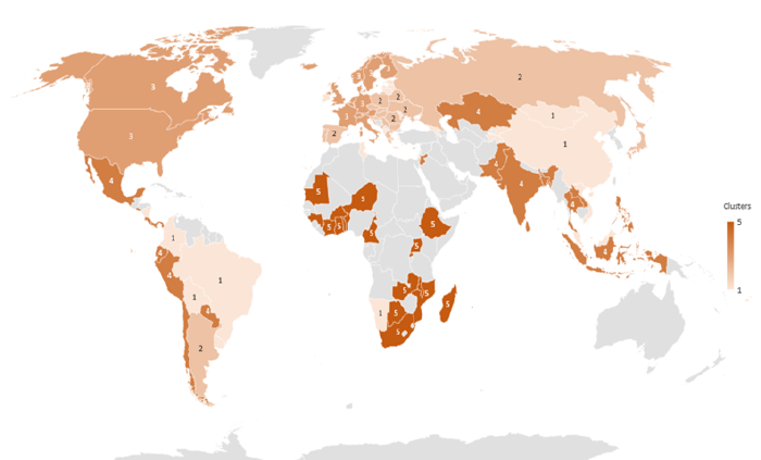
Figure 4. Differences across clusters’ averages

Source: Authors.

Note: centroids of each cluster relative value in terms of the maximum and minimum values of the different clustering variables.

It is also important to note that, as in any international classification, there are countries that do not perfectly fit their assigned groups. The most notable case in our taxonomy is Ireland, which is the country with the highest income and the highest wealth growth rate of the rich among C1 countries. Therefore, Ireland is the last country in joining C1 according to the agglomeration schedule (See Appendix 2).

These results are interesting, as the classification clearly identifies the main peculiarities of each group regarding the recent explanation of inequality. For example, in the case of Latin American countries (Cluster 4), the taxonomical analysis highlights that, beyond the fluctuations in the tails of the income distribution, low tax collection is the main differentiating element of this group. Moreover, the main inequality challenge of African and Middle Eastern countries (Cluster 5) is reducing the income gap between the top 10% and the bottom 40%. And in the case of European Union countries and the USA (Cluster 3), the key feature of inequality is the significant increase of wealth for the richest population —the top 1%.

5. Conclusions

Over recent years, inequality has become the focus of public attention for several reasons, including the growing interest in “confronting inequalities,” the increase of within-country inequality, and the connection between inequality and less sustained growth, among others. The uneven distribution of income and wealth has caused an increasing social discontent that threatens to destabilize democracies and fosters a variety of economic, social, political, and ecological injustice.

Fighting inequality is an essential component in the quest for sustainable development, as recognized by the United Nations’ 2030 Agenda for Sustainable Development. Accordingly, not only is there an urging need to reduce economic inequalities, but also to better examine and to assess the aim of reducing the inequality gap around the world.

Our assessment has provided insights into this matter from a multidimensional approach about economic inequality. We acknowledge the need to critically look at income and wealth data and we assume that there is no single yardstick capable of conveying a full picture of inequality. Therefore, we consider a broader view through different facets of economic inequalities, including a global assessment of this phenomenon.

The aim of this paper is to build an international and multidimensional taxonomy of economic inequality that takes into account five main dimensions: the adjusted household income, the capacity of the State to tackle inequalities, the income growth of the poor, the wealth growth of the rich, and the differences in the tails of the distribution (between the rich and the poor). By means of a hierarchical cluster analysis, we identify five groups of countries with similar inequality features over the last years:

• Cluster 1 is a heterogeneous group of countries characterized by high income growth rates for the bottom 40% of the population, yet they have low per capita incomes, moderate Palma ratios, and tax revenues.
• Cluster 2 consists of countries with low (and in some cases even negative) growth rates of both the income of the poor and the wealth of the rich. Moreover, tax revenues are comparatively high and Palma ratios are low.
• Cluster 3 is made up of developed countries with high wealth growth rates of the rich and low Palma ratios.
• Cluster 4 consists of countries with very low tax revenues, medium income levels, and high Palma ratios. Nevertheless, income of the poor is growing at positive rates whereas the wealth growth of the rich is slightly negative for many countries.
• Cluster 5 consists of countries with very high Palma ratios and very low tax revenues. However, the income of the poor is growing at positive rates (for most of the countries) whereas the wealth growth of the rich is slightly negative for some countries.

Moreover, this international classification shows that, despite national and regional specificities, both developed and developing countries face important hurdles in addressing national economic inequality. Hence, these hurdles deserve to be thoroughly discussed to prevent painting all countries with the same brush. Nonetheless, we acknowledge that we have carried out a partial assessment of inequality, limited to its economic dimension and thus, neglecting other social and environmental variables. The aim is to address this constraint in future research.

The intended contribution of the paper is to demonstrate that more work on the complexity of global inequalities is required since both advanced economies and the Global South share significant difficulties for reducing economic inequalities. Therefore, there is no need for a “one size fits all” international strategy to tackle global inequality. Conversely, the evidence suggests that there is a need of multiple and simultaneous strategies to effectively address the different patterns of inequality that we have identified around the world.

There are, however, some constraints to our analyses, especially in terms of quality and availability of the inequality data. Moreover, as in any international classification, there are countries that do not perfectly fit in our taxonomy and require detailed case-studies. Besides, it is important to bear in mind the descriptive nature of cluster analysis, which implies that it needs to be complemented with other causal analysis that shed light on the different drivers of income inequalities around the world.

All in all, this piece of research aims to serve as a foundation for further progress and to inspire other researchers in the multidimensional measurement of the global issue of income inequalities.

6. References

Alvaredo, F., Chancel, L., Piketty, T. Saez, E. and Zucman, G. (2018). The Elephant Curve of Global Inequality and Growth, AEA Papers and Proceedings;108:103-108 https://doi.org/10.1257/pandp.20181073

Arrighi, G. 2007. Adam Smith in Beijing: lineages of the twenty-first century, Verso. London.

Atkinson, A. B. (1970). On the measurement of inequality, Journal of Economic Theory (2),244-263

Atkinson, A.B. Measuring Top Incomes: Methodological Issues. In: A. B. Atkinson and T. Piketty (eds.): Top Incomes over the Twentieth Century: A Contrast Between Continental European and English-Speaking Countries. Oxford University Press; 2007. p. 18-42.

Atkinson, A.B. Inequality. What can be done? Cambridge: Harvard University Press; 2015.

Atkinson, A. B. and Bourguignon F. (eds) Handbook of Income Distribution. Volume 2. Pages 1-2251. Amsterdam: North-Holland; 2015.

Atkinson, A.B., Piketty, T. and Saez, E. Top Incomes in the Long Run of History, Journal of Economic Literature 2011; 49:3-71.

Bourguignon, F. Spreading the Wealth, Finance and Development 2018; 55:22-24.

Brei, M; Ferri, G. and Gambacorta, F. Financial structure and income inequality, Bank for International Settlements Working Papers No 756; 2018.

Calinski, T. and Harabasz, J. A dendrite method for cluster analysis. Communications in Statistics - Theory and Methods 1974; 3: 1-27.

Carsten, J. & van Kersbergen, K. Politics of Inequality, Palgrave. NY, 2017.

Chang, H-J. 23 Things they don’t tell you about capitalism. London: Penguin Books; 2011.

Cobham, A., Schlögl, L., Sumner. A. Inequality and the Tails: the Palma Proposition and Ratio. Global Policy 2016, 7(1):25-36.

Credit Suisse Research Institute Global Wealth Report 2012. Zürich, Switzerland: Credit Suisse AG; 2012.

Credit Suisse Research Institute. Global Wealth Report 2014. Zürich, Switzerland: Credit Suisse AG., 2015.

Domínguez Martín, R. 2014. “International Cooperation Perspectives and Sustainable Development After 2015”. Revista Internacional de Cooperación y Desarrollo 1 (2):5-32 https://revistas.usb.edu.co/index.php/Cooperacion/article/view/2241/1961

Dos Santos, T. 2011. Imperialismo y dependencia. Biblioteca Ayacucho, Caracas

Everitt, B.S., Landau, S., Leese, M. and Stahl, D. Cluster analysis. Chichester: John Wiley and Sons; 2011.

Fields. G. Distribution and Development: A New Look at the Developing World. Cambridge, Massachusetts: The MIT Press; 2002.

Fleurbaey, M. and Klasen, S. Inequalities and social progress in the future, in World Social Science Report, 2016: Challenging inequalities; pathways to a just world. IDS and UNESCO, Paris; 2016.

Gaventa, J. Consequences and futures of inequalities (an introduction to Part II), in World Social Science Report, 2016: Challenging inequalities; pathways to a just world. IDS and UNESCO, Paris; 2016.

Gouda, T. The global concentration of wealth, Cambridge Journal of Economics 2018; 42: 95-115. doi: 10.1093/cje/bex020

Ibarra, C. and Ros, J.: The decline of the labor income share in Mexico, 1990-2015, World Development 2019; 122: 570-584.

ICTD/UNU-WIDER: Government Revenue Dataset. (2020) https://www.wider.unu.edu/project/government-revenue-dataset

Josa, I. and Aguado, A. Measuring Unidimensional Inequality: Practical Framework for the Choice of an Appropriate Measure. Social Indicators Research; 2020. https://doi.org/10.1007/s11205-020-02268-0

Kakwani, N., Khandker; S. and Son, H. Pro-poor growth: concepts and measurement with country case studies”, Working Papers 1, International Policy Centre for Inclusive Growth; 2004.

Kaldor, N.: Collected economic essays 8. Reports on taxation 2: papers relating to foreign governments. Holmes and Meier, NY; 1980.

Kanbur, R.: Inequality in a global perspective, Oxford Review of Economic Policy 2019; 35(3): 431-444.

Keeley, B.: Income Inequality: The Gap between Rich and Poor, OECD Insights, Paris: OECD Publishing; 2015.

Keynes, J.M.: The General Theory Of Employment, Interest And Money, Cambridge University Press: Cambridge; 1936.

Lahoti, R., Jayadev, A. and Reddy, S.: The Global Consumption and Income Project (GCIP): An Overview, LIS Working papers 655, LIS Cross-National Data Center; 2016.

Lakner, C. and Milanovic, B.: Global Income Distribution: From the Fall of the Berlin Wall to the Great Recession, The World Bank Economic Review 2016; 30(2): 203-232.

La Porta, R. and Shleifer. A. Informality and Development, Journal of Economic Perspectives 2014; 28(3): 109-126.

Long, C. and Miller, M. Taxation and the Sustainable Development Goals. Do good things come to those who tax more?, ODI briefing paper. Overseas Development Institute; 2017.

Milanovic, B. Global Inequality Recalculated and Updated: The Effect of New PPP Estimates on Global Inequality and 2005 Estimates. The Journal of Economic Inequality 2012; 10: 1–18.

Milanovic, B. Global Inequality. A New Approach for the Age of Globalization, Harvard University Press, Cambridge; 2016.

Milligan G.W. and Cooper, M. An examination of procedures for determining the number of clusters in a data set. Psychometrika 1985; 50(2): 159-179.

Mooi, E. and Sarstedt, M.: A concise guide to market research. Berlin. Springer-Verlag; 2011.

Mueller, J.: War Has Almost Ceased to Exist: An Assessment. Political Science Quarterly 2009; 124(2): 297-321.

Mundell, R. Capital Mobility and Stabilization Policy under Fixed and Flexible Exchange Rates. The Canadian Journal of Economics and Political Science 1963;29(4): 475-485.

Nino-Zarazúa, M., Roope, L, and Tarp, F. Global inequality: relatively lower, absolutely. Review of Income and Wealth 2017;63(4): 661-684.

OECD. Illicit Financial Flows from Developing Countries: Measuring OECD Responses. Paris, OECD; 2014.

Ostry, J., Loungani, P. and Berg, A. Confronting Inequality. How Societies Can Choose Inclusive Growth. Columbia University Press, New York; 2019.

Palma, J.G. Behind the Seven Veils of Inequality. What if it’s all about the Struggle within just One Half of the Population over just One Half of the National Income?, Development and Change 2019; 50(5): 1133-1213.

Palma, J. G. Has the Income Share of the Middle and Upper-middle Been Stable around the ‘50/50 Rule’, or Has it Converged towards that Level? The ‘Palma Ratio’ Revisited. Development and Change 2014; 45(6): 1416-1448.

Piketty, T. Capital in the Twenty-first Century. The Belknap Press of Harvard University Press, Cambridge; 2014.

Ravallion, M. Inequality and Globalization: A Review Essay, Journal of Economic Literature 2018; 56(2), 620-642.

Rawls, J. A Theory of Justice. The Belknap Press of Harvard University Press, Cambridge; 1971.

Roemer, J E and Trannoy, A. Equality of opportunity, in A B Atkinson and F Bourguignon (eds), Handbook of Income Distribution vol 2A, Amsterdam: North-Holland; 2015.

Scheidel, W.: The Great Leveler. Violence and the History of Inequality from the Stone Age to theTwenty-First Century, Princeton University Press, New Jersey; 2016.

Stiglitz, J. Distribution of Income and Wealth Among Individuals, Econometrica 1969; 37(3): 382-397.

Stiglitz, J. Where modern macroeconomics went wrong, Oxford Review of Economic Policy 2018; 34(1-2): 70-106.

UNDESA. Note on Income Inequality Data. Global Dialogue for Social Development Branch Emerging Issues and Trends Section. New York; 2018.

United Nations. Transforming our world: the 2030 Agenda for Sustainable Development. Resolution adopted by the General Assembly on 25 September 2015. A/RES/70/1. New York; 2015.

UNDP. Human Development Report 2019. Beyond income, beyond averages, beyond today: Inequalities in human development in the 21st century. New York.

Wallerstein, I. 2004. World-systems analysis: an introduction. Duke University Press, Durham and London.

World Bank. World databank 2020 http://data.worldbank.org, accessed 19 August 2019

APPENDICES

Appendix 1. Descriptive statistics of the data set

	N	Minimum	Maximum	Mean	Std. Deviation
Income_pc_adj	105	47,3	2154,99	641,6597	534,03124
Palma	105	0,88	9,59	3,0287	1,96871
Growth_40	105	-8,35	9,13	1,7075	2,68335
Growth_rich	101	-13,8	14,1	0,1327	3,46278
Tax_revenue	105	5,59	45,9	24,7105	10,12828
Valid N (listwise)	101

Source: Authors.

Appendix 2. Agglomeration schedule

Stage	Cluster Combined		Coefficients	Stage Cluster First Appears		Next Stage
	Cluster 1	Cluster 2		Cluster 1	Cluster 2
1	35	68	0,001	0	0	51
2	25	74	0,002	0	0	50
3	51	52	0,004	0	0	49
4	3	90	0,006	0	0	35
5	7	32	0,008	0	0	18
6	1	49	0,011	0	0	35
7	24	31	0,013	0	0	30
8	27	40	0,016	0	0	13
9	64	92	0,019	0	0	60
10	14	80	0,022	0	0	25
11	16	72	0,027	0	0	55
12	5	71	0,031	0	0	69
13	27	75	0,036	8	0	28
14	23	76	0,04	0	0	21
15	67	69	0,045	0	0	33
16	9	61	0,05	0	0	44
17	13	37	0,055	0	0	46
18	7	88	0,061	5	0	70
19	39	66	0,067	0	0	70
20	89	98	0,073	0	0	74
21	23	79	0,08	14	0	59
22	77	82	0,086	0	0	47
23	41	50	0,093	0	0	56
24	81	96	0,099	0	0	29
25	8	14	0,106	0	10	48
26	54	95	0,113	0	0	58
27	18	100	0,121	0	0	62
28	27	86	0,128	13	0	56
29	63	81	0,136	0	24	68
30	4	24	0,144	0	7	72
31	83	85	0,152	0	0	64
32	12	78	0,16	0	0	68
33	33	67	0,169	0	15	62
34	62	94	0,179	0	0	63
35	1	3	0,188	6	4	53
36	73	91	0,199	0	0	42
37	29	87	0,209	0	0	58
38	6	44	0,22	0	0	64
39	15	97	0,231	0	0	52
40	48	60	0,243	0	0	50
41	65	93	0,255	0	0	80
42	19	73	0,267	0	36	55
43	2	21	0,279	0	0	47
44	9	11	0,292	16	0	71
45	26	58	0,306	0	0	51
46	13	20	0,322	17	0	85
47	2	77	0,338	43	22	61
48	8	55	0,355	25	0	60
49	28	51	0,372	0	3	83
50	25	48	0,39	2	40	76
51	26	35	0,409	45	1	57
52	15	34	0,428	39	0	78
53	1	30	0,448	35	0	63
54	10	84	0,468	0	0	94
55	16	19	0,491	11	42	67
56	27	41	0,518	28	23	69
57	26	59	0,546	51	0	73
58	29	54	0,577	37	26	73
59	23	38	0,61	21	0	61
60	8	64	0,644	48	9	66
61	2	23	0,682	47	59	75
62	18	33	0,721	27	33	79
63	1	62	0,761	53	34	79
64	6	83	0,803	38	31	75
65	17	56	0,848	0	0	83
66	8	101	0,896	60	0	85
67	16	47	0,95	55	0	87
68	12	63	1,004	32	29	82
69	5	27	1,061	12	56	76
70	7	39	1,117	18	19	90
71	9	99	1,175	44	0	80
72	4	45	1,25	30	0	90
73	26	29	1,337	57	58	86
74	70	89	1,425	0	20	84
75	2	6	1,515	61	64	82
76	5	25	1,61	69	50	87
77	22	46	1,708	0	0	88
78	15	53	1,813	52	0	84
79	1	18	1,93	63	62	89
80	9	65	2,049	71	41	89
81	43	57	2,211	0	0	96
82	2	12	2,373	75	68	95
83	17	28	2,537	65	49	93
84	15	70	2,703	78	74	92
85	8	13	2,89	66	46	91
86	26	42	3,085	73	0	91
87	5	16	3,301	76	67	97
88	22	36	3,522	77	0	95
89	1	9	3,744	79	80	93
90	4	7	3,968	72	70	92
91	8	26	4,303	85	86	94
92	4	15	4,666	90	84	98
93	1	17	5,084	89	83	96
94	8	10	5,558	91	54	99
95	2	22	6,064	82	88	98
96	1	43	6,697	93	81	97
97	1	5	7,606	96	87	99
98	2	4	9,614	95	92	100
99	1	8	12,625	97	94	100
100	1	2	22,232	99	98	0

Source: Authors.

Appendix 3. Cluster membership of developing countries

Country	Cluster membership	Income_pc_adj	Palma	Growth_40	Growth_rich	Tax revenue
Albania	1	273.03	2.50	1.16	-0.2	24.09
Armenia	1	197.75	2.61	1.76	0	21.57
Bolivia	1	414.91	3.00	2.63	0	31.3
Brazil	1	481.35	3.39	1.7	-1.4	33.71
China	1	690.36	3.92	9.13	0.2	24.08
Colombia	1	326.51	3.93	3.48	-1.3	20.1
Estonia	1	804.74	1.49	6.15	2	33.71
Fiji	1	257.08	3.76	1.17	0	25.48
Georgia	1	237.63	3.07	4.48	0	25.23
Ireland	1	1,306.16	1.31	1.69	14.1	23.16
Kyrgyz Republic	1	140.69	2.41	0.86	-0.1	25.3
Latvia	1	638.60	1.51	7.52	0.3	29.01
Lithuania	1	673.45	1.47	6.65	-0.5	29.18
Malaysia	1	847.59	2.61	8.3	-0.9	14.29
Malta	1	242.06	1.05	3.57	13.8	32.77
Moldova	1	260.33	2.41	2.61	0	31.62
Mongolia	1	456.66	3.11	1.74	0.6	22.14
Namibia	1	359.42	4.47	5.73	-2.8	33.12
Nicaragua	1	288.89	2.67	5.64	0	22.32
North Macedonia	1	383.20	2.72	6.45	-0.1	25.22
Tajikistan	1	89.22	2.58	2.3	-0.1	22
Tunisia	1	468.11	5.31	4.97	-0.9	30.26
Turkey	1	613.56	2.54	2.53	-0.4	25.09
Uruguay	1	668.35	2.03	3.22	-6	28.87
Vietnam	1	385.92	3.42	4.92	-0.1	18.22
Argentina	2	704.36	2.09	0.77	-1.1	31.99
Belarus	2	948.29	2.43	1.09	0	35.58
Bulgaria	2	553.27	1.57	0.43	0.4	28.88
Croatia	2	509.50	1.19	0.48	-1.6	34.8
Cyprus	2	1,382.04	1.62	-4.34	-6.4	24.24
Czech Republic	2	827.73	0.91	1.42	-0.4	33.35
Greece	2	668.31	1.49	-8.35	-6.3	36.4
Hungary	2	595.80	1.15	1.19	1.4	39.01
Israel	2	1,033.74	2.01	1.54	2.2	31.32
Japan	2	1,395.46	1.18	1.1	-13.8	30.85
Montenegro	2	442.91	2.20	-2.73	-0.4	36.36
Poland	2	727.61	1.28	2.54	0.3	32.44
Portugal	2	788.73	1.55	-0.87	-3.8	34.56
Romania	2	301.55	1.52	0.06	-0.6	27.61
Russian Federation	2	740.57	1.30	1.62	0	29.2
Serbia	2	337.40	1.47	-1.7	-0.7	34.62
Slovak Republic	2	726.46	0.96	-0.62	-2	32.31
Slovenia	2	1,010.89	0.91	-0.77	1.2	36.32
Spain	2	1,089.40	1.51	-2.16	1.3	33.81
Ukraine	2	407.79	2.30	-0.83	-0.1	34.45
Austria	3	1,698.64	1.14	-0.47	-1.6	43.67
Belgium	3	1,454.85	0.97	0.57	4.6	44.81
Canada	3	1,781.28	1.33	-0.24	3.5	32.12
Denmark	3	1,548.69	1.08	0.56	-1.7	45.9
Finland	3	1,496.27	0.96	0.53	-0.4	43.93
France	3	1,568.08	1.29	0.74	4.5	45.22
Germany	3	1,628.74	1.21	-0.18	-0.6	37.07
Iceland	3	1,475.59	0.88	-0.13	6.3	36.67
Italy	3	1,172.84	1.41	-2.14	-6.9	43.29
Luxembourg	3	2,154.99	1.24	-2.14	-5.1	36.83
Netherlands	3	1,457.35	1.04	0.95	8.7	37.36
Norway	3	2,097.53	0.91	2.12	10.3	38.46
Sweden	3	1,602.41	0.98	1.8	4.9	43.28
Switzerland	3	2,017.40	1.19	0.98	4.2	27.34
United Kingdom	3	1,498.23	1.29	0.42	2	32.53
United States	3	1,954.67	1.95	1.31	5.7	26.23
Bangladesh	4	166.41	2.36	1.35	0	7.93
Chile	4	730.02	3.29	4.67	-2	18.86
Costa Rica	4	711.74	3.01	2.04	-1.7	13.39
Ecuador	4	362.87	2.47	2.41	0.1	15.55
El Salvador	4	249.93	2.10	4.12	0.1	15.07
India	4	181.91	2.58	3.69	0	16.48
Indonesia	4	253.91	3.63	4.77	-0.3	10.75
Jordan	4	1,063.98	3.70	0.75	0.1	15.45
Kazakhstan	4	606.71	2.38	-0.02	-0.4	15.89
Lao PDR	4	202.27	3.47	3.39	0.2	13.77
Mexico	4	350.26	2.99	0.51	-1.4	17.4
Pakistan	4	155.16	2.30	2.72	0	9.99
Panama	4	659.72	3.34	4.65	-1.5	15.5
Paraguay	4	510.13	3.46	3.21	0	14.25
Peru	4	345.33	2.33	1.72	0	14.72
Philippines	4	236.62	2.65	5.12	0.2	16.63
Sri Lanka	4	309.83	2.66	4.24	0	12.52
Thailand	4	676.92	3.46	2.51	0.1	18.76
Benin	5	95.75	6.39	0.28	0.1	15.89
Botswana	5	482.52	9.59	0.42	-0.4	23.23
Burkina Faso	5	113.85	5.23	5.84	0	14.09
Cameroon	5	184.96	7.07	1.36	0	15.75
Côte d’Ivoire	5	185.34	6.31	5.95	0.1	15.26
Egypt, Arab Rep.	5	250.26	3.95	0.48	-0.1	12.52
Ethiopia	5	122.82	4.91	0.35	0	8.76
Ghana	5	178.94	5.18	-0.2	0	15.01
Guinea	5	110.59	5.03	4.14	0	13.07
Iran, Islamic Rep.	5	1,050.73	5.58	-3.15	-0.5	7.12
Madagascar	5	47.30	6.16	-0.28	0	10.39
Malawi	5	52.95	6.59	3.05	0	15.16
Mauritania	5	221.63	4.92	2.28	0	15.16
Mauritius	5	421.83	5.23	0.49	-2.8	18.96
Mozambique	5	77.66	6.51	1.87	0	21.73
Niger	5	101.43	5.15	-0.06	0	16.04
Rwanda	5	95.37	7.31	0.31	0	15.67
South Africa	5	381.14	8.96	-1.34	-0.3	29.44
State of Palestine	5	318.53	5.20	-0.89	-0.4	5.59
Togo	5	132.35	6.96	2.76	0	21.4
Uganda	5	124.98	6.01	-2.2	0	11.68
Zambia	5	140.92	8.41	-0.59	0	14.42

Source: Authors.

---